Part 5: The p-Machine (intro)

Previously: Intro, Running Apple Pascal on a modern Mac, The Editor, The Filesystem, Text Files, Code Files

What is the p-Machine, and why is it like that?

Before we can go into greater detail about what the code in our example (and other programs) actually does, we’re going to need a little background on what the p-Machine architecture is, and why it has some of the features that it has.

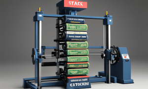
The p-Machine is a Stack Machine

Essentially all modern CPU designs are designed around a register-centric architecture. They have many general-purpose registers, and most operations are done register-to-register. This is especially true in RISC architectures, where typically the ALU and other logic units can only access registers, not main memory.

Even in CISC architectures like x86, where one or more operands can be from memory, register-to-register operations are preferred, in the sense that they’re much faster than going to main memory. This sort of design is important in order to get the best possible performance.

But that sophistication comes at a cost – these processors are very complicated, internally. What if you really wanted to simplify the internal design of the processor, possibly at the expense of performance. Say, if you were expecting to write an emulator for it in assembly language? Well then, you might design a Stack Machine.The p-Machine has zero general purpose registers, and very few addressing modes, even compared to contemporary microprocessors of the 1970s.

But why would you want that?

Simplicity of implementation is definitely one reason. Given the desire for the p-System to run on all hardware, everywhere, you really want a design that requires very little in the way of specific processor features. And, again – you’re going to be writing this interpreter in Assembly code, so you really want to be able to do it in as little code as possible.

Another reason is compactness. Nearly every arithmetic or logical operation gets its operands from the stack and stores results to the stack. There’s no need encode those arguments in the instructions, so those instructions are all single bytes. A lot of code samples are literally half the size or smaller compared to native code. Given the overhead of having the OS resident in memory too, this is a huge help for smaller systems like the Apple II. Don’t forget that floppy disks of the time only held up to a few hundred kB or so.

Stack Machines were everywhere in the 1980s and 1990s, especially in games

These twin advantages of fast porting and small program size were really useful in another part of the home computer industry: video games.

Infocom created a virtual machine architecture called the Z-machine, inspired by the p-System, which was how they ported Zork (and later adventure games) to all of the zoo of different home computers of the time. There are many other examples, including AGI, the Adventure Game Interpreter used by Sierra Online for their graphical adventure programs, SidTran which was used in Microprose’s early simulator games, etc.

Similarly, the Java Virtual Machine chose a stack-based design in order to optimize download time on a mostly dial-up Internet at the time.

How does a Stack Machine work, then?

There are some similarities to RISC, in that stack machines also use a load, calculate, store paradigm. It’s just that the “loads” go onto a stack, and most instructions get their arguments from the stack. If you’ve ever used an HP calculator with RPN operation, or FORTH, you will be on familiar ground, here. If not, here’s a quick example:

Say you want to calculate (2+3)*4. On the p-Machine, you could do it like this. The stack is represented below with the “top” to the right.

Instruction	Description	Stack Contents [bottom, …, top]
SLDC 4	Load value 4 on to stack	[4]
SLDC 3	Load value 3 on to stack	[4, 3]
SLDC 2	Load value 2 on to stack	[4, 3, 2]
ADI	Add top two values on the stack, push result to stack	[4, 5]
MPI	Multiply top two values on the stack, push result to stack	[20]

Note that you can also do this by adding 2+3 first, then pushing 4 and multiplying. I did it this way because the stack diagram is more interesting this way, and so that the HP calculator super-fans don’t come after me in the comments 🙂

The p-Machine (version II)

The version of the p-Machine used in Apple Pascal is closely-based on UCSD version II.0. There are major differences between the various editions of the p-Machine, so I’m going to stick to describing version II, for now. I hope to expand to cover the IV release at some point.

Side note: the Internal Architecture Guide for version IV (from Softech) is readily-available on the Internet, but earlier versions are not. If you happen to have a copy of the Internal Architecture Guide for UCSD versions I, II, or III (if they indeed exist), I would dearly love to see them. Like, I would definitely pay you to ship them to me, for scanning and uploading to the Internet Archive.

General organization

The nominal word size for the p-Machine is 16 bits. The endianness of memory is up to each implementation to decide. Typically, you’d want to match whatever the hardware expects.

Registers

The p-Machine has 8 registers, all of which store addresses in main memory. Every one of these is nominally a 16-bit pointer to a location in main memory:

name	description
SP	Stack Pointer
IPC	Interpreter Program Counter
SEG	Points to the Procedure Dictionary of the segment to which the currently-executing procedure belongs
JTAB	Points to the table of attributes and jump table of the current segment
KP	Stack Pointer – starts high, grows down toward heap
MP	MarkStack pointer – points into the current activation record. This is where the local variables are
NP	New Pointer – points to the top of the heap. Grows up from high memory toward the stack
BASE	Points to the activation record of the most recently-invoked base procedure (level 0). Globals live here

Opcodes

All opcodes in the p-Machine are a single byte, with sometimes a number of following bytes as arguments. I’m not going to duplicate the entire opcode table here, but I’ll cover some of the general categories, and some interesting choices.

SLDC: The most-important Opcode (at least by number of variants!)

Fully half of the opcodes in the p-Machine are for a single operation. SDLC x loads a constant value onto the stack. Loading a constant is one of the most common operations, so it makes sense to make all of these one-byte instructions. I find it amusing that the opcode for SLDC 0 is just 0, and so on down the line to SLDC 127, which is 127, naturally. This allows you to push any constant from 0 to 127 onto the stack with a single instruction. There is a related opcode for loading an arbitrary word onto the stack, LDCI x, which is 3 bytes, one for the opcode, and 2 for the 16-bit word to push.

Arithmetic and logic operations

For arithmetic, you have add, subtract, multiply, divide, square, absolute value, and negate for integer and real values on the top of the stack. These are all single-byte instructions, with no arguments. There are comparison operations for integers, reals, and strings. These are all two-byte instructions, where the second byte specifies the type to compare.

Jumps

Jumps are two bytes long. And this one is a bit odd: if the offset is positive, it’s just added to IPC as you’d expect. If it’s negative, it’s used to index into the jump table pointed to by the JTAB register. This means that any jump that is either backward or more than 255 bytes forward is done through an indirect lookup.

Weird Pascal stuff

You knew this was coming, right? Since the p-System was originally designed to support Pascal, there are some wacky operations that are clearly designed specifically to support Pascal programs. You’ve already seen LSA, which is designed to push the address of a Pascal-style string (length byte, followed by characters) onto the stack. This single-byte instruction does the equivalent of reading a string table pointer, incrementing it by a byte value, and then pushing it onto the stack.

Another fun quirk is that there are dedicated instructions for comparing, setting, and copying sets, byte arrays, and records. Each of these operations is defined in terms of the Pascal semantics, though I imagine they’re at least somewhat generally useful.

And then there are the memory store operations. These are deeply influenced by Pascal’s scoping rules. There are instructions for loading and storing to local variables, to do the same with global variables (indexed through the BASE register), and for intermediate variables from other lexical scopes (by walking the activation records on the stack).

Then there are a few opcodes that call routines either in the OS, or other Units in the program.

What’s next?

I think what’s next is going back to that first code example, fully disassembling it, and walking through it to see how it works. For that, we’re going to need a disassembler…